J4 - J5 perturbations

cristiapi

New member
Joined
May 26, 2014
Messages
222
Reaction score
0
Points
0
Location
Ancona
If I calculate the J2 perturbation for geodetic latitude= 30° (geocentric latitude= 29.8435°) and longitude= 50° (geocentric Cartesian coordinates [m]=
X= 3776163.03059535, Y= 4500255.85793345, Z= 3370373.73538364),
I get (m/s2):
gx= 0.00166079432943605
gy= 0.00197925760866551
gz= -0.0109643334779438
g= 0.0112646485565111


[With your formulas I get:
a2_radial= 0.00321510045644651
a2_north= 0.0124461432971332
a2= 0.0128547016269463.
Even if the difference is not too big, I expected to get exactly the same result. Where am I wrong?]


EDIT: oops! I get exactly the same result. It helped a lot! Thank you very much.
Now I'm trying to get X, Y, Z from your formulas...
 
Last edited:

martins

Orbiter Founder
Orbiter Founder
Joined
Mar 31, 2008
Messages
2,448
Reaction score
462
Points
83
Website
orbit.medphys.ucl.ac.uk
I don't know how you computed the results, but looking at the Wikipedia article, its equations in spherical coordinates for the J2 contribution (Eq. 12) look the same as mine (Eq. 6) when you take into account their conversion of the J2 coefficient (Jn -> \tilde{Jn} = Jn/G/M/R^n)

There does seem to be something wrong in the Wiki article though. Eq. 12 is supposed to show the force components, but the RHS dimensions are that of an acceleration ([J2/r^4] = m^5 s^-2 m^-4 = m/s^2)
 

cristiapi

New member
Joined
May 26, 2014
Messages
222
Reaction score
0
Points
0
Location
Ancona
I don't use equations 12, but I can confirm that Eq. 13 are accelerations, not force.

Back to my problem, if I use Ftheta and Fr (as in your pdf) I need to calculate sqrt(Ftheta^2 + Fr^2) and then I must convert the result in ECI reference frame, very lengthy procedure.
Is there any chance to get directly the X, Y, Z components?
 

martins

Orbiter Founder
Orbiter Founder
Joined
Mar 31, 2008
Messages
2,448
Reaction score
462
Points
83
Website
orbit.medphys.ucl.ac.uk
Isn't that just the standard polar -> cartesian conversion? You know,

x = r sin f cos p
y = r sin f sin p
z = r cos f
 

cristiapi

New member
Joined
May 26, 2014
Messages
222
Reaction score
0
Points
0
Location
Ancona
If f is the geocentric latitude and p is the longitude it should be:
x = r cos f cos p
y = r cos f sin p
z = r sin f
but it doesn't work, because I get
a2x= 0.00628056431951873
a2y= 0.00748488509130546
a2z= 0.00560565019422803

while according to Eq. 13 the correct result is
x= 0.00166079432943605
y= 0.00197925760866551
z= -0.0109643334779438
 

Thorsten

Active member
Joined
Dec 7, 2013
Messages
785
Reaction score
56
Points
43
but I would also add J4 and possibly J5 too.

Are you aware that a lot of other effects (3rd body perturbations, solar radiation pressure, residual atmosphere drag,...) are going to be much larger than these? And that some of these come with fairly large uncertainties?

So while it is an interesting mathematical exercise, it doesn't actually add accuracy.
 

cristiapi

New member
Joined
May 26, 2014
Messages
222
Reaction score
0
Points
0
Location
Ancona
If we take a look at this graph:

SFERA2_R_J2+J3.png


we see that adding the J3 perturbation greatly improves the result (I take SGP4 as the correct result).
I suspect that adding also J4, the result is further significantly improved. It's surely worth trying.
 

Thorsten

Active member
Joined
Dec 7, 2013
Messages
785
Reaction score
56
Points
43
suspect that adding also J4, the result is further significantly improved.

There's no need to suspect things you can just look up or calculate, and if what you say were true, the expansion in harmonics would be pointless (the whole point is that each term gets progressively smaller so you can terminate the series early). Just a quick assembly of numbers for satellites on GPS orbits pulled from here

Over the course of three days, the orbit deviates from an analytical 2-body orbit by about

14000 m due to J2
1500 m due to all higher harmonics
3000 m due to solar and lunar gravity
800 m due to solar radiation pressure

So even the whole sum of J3, J4, J5... is not the first sub-leading effect below J2, it's solar and lunar gravity for that orbit. What's not on the page (but what I have computed by my own code) is that J3 already accounts for the majority of the 1500 m - so also the solar radiation pressure is larger than J4 and higher.

But the solar radiation pressure depends on things like solar activity or the shape and orientation of your spacecraft - which you can't easily know or predict in advance. So this is the term that sets your uncertainty and you have to compensate for via stationkeeping - the few meters the yet higher harmonics actually cause don't matter much.

In any case - please don't let me keep you from exploring an interesting math problem - but be aware that accuracy isn't set by J4 and higher.
 

MontBlanc2012

Active member
Joined
Aug 13, 2017
Messages
138
Reaction score
26
Points
28
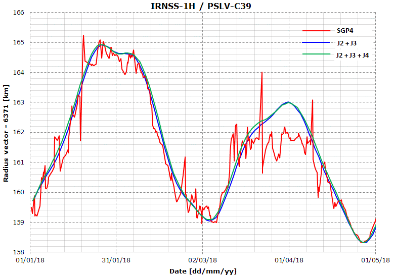
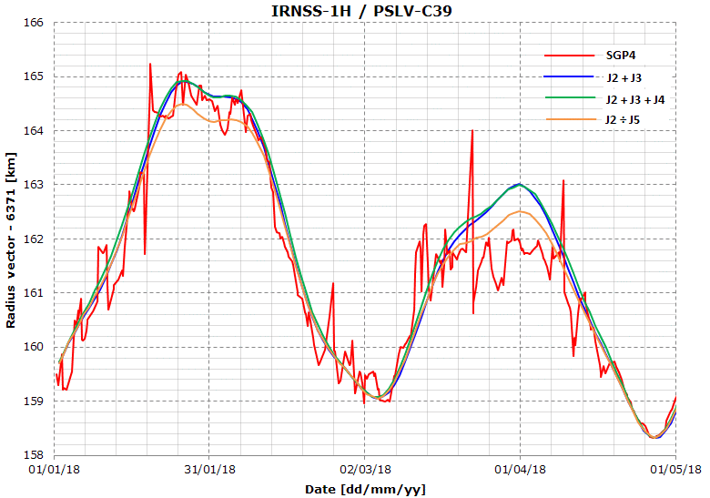
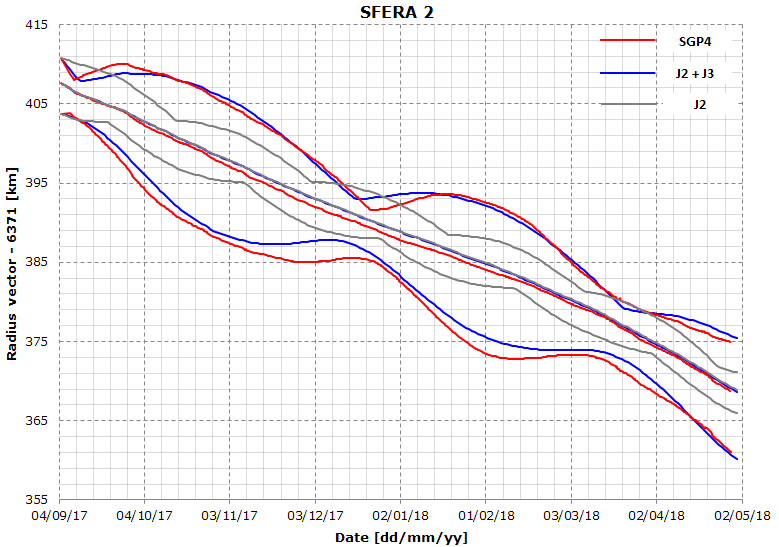
n my simulation, I’m currently using J2 + J3 perturbations (Fx, Fy, Fz) as depicted on this page: https://en.wikipedia.org/wiki/Geopot...geneous_sphere
but I would also add J4 and possibly J5 too.
Unfortunately, I don’t know how to go from u= J2 * P2(sin theta) / r3 to Fx, Fy, Fz. Please, could anyone explain?

cristiapi:

The wikipedia article that you referenced (Geopotential model) contains the following expression for the Earth's gravitational potential:

[math]u = -\frac{\mu}{r} + \sum_{n=2}^{N}\frac{J_n\,P_n(\sin\theta)}{r^{n+1}}+\dots[/math]
where [imath]\sin\theta = z/r[/imath] and [imath]r^2 = x^2 + y^2 + z^2[/imath]. All of the [imath]J_n[/imath] are just constants and the [imath]P_n(\xi)[/imath] are just the Legendre polynomials (Legendre polynomials).

The first term in this expression is the one that gives rise to the usual inverse square law for gravity. The terms involving the [imath]J_n[/imath] are the 'zonal' terms of the expansion. There are other 'tesseral' terms, but we can gloss over these. The first 'zonal' term is, as you point out:

[math]\Delta u_2 = \frac{J_2\,P_2(z/r)}{r^3}[/math]
where, again, [imath]r[/imath] is a function of the [imath]x[/imath], [imath]y[/imath] and [imath]z[/imath] Earth-centred equatorial coordinates. From this contribution to the Earth's gravitational potential we can calculate the corresponding contribution to the gravitational acceleration by substituting [imath]r\to\sqrt{x^2 + y^2 + z^2}[/imath] calculating:

[math]\begin{aligned} \Delta F_{2,x} &= -\frac{\partial \,\Delta u_2}{\partial x} \\ \Delta F_{2,y} &= -\frac{\partial \,\Delta u_2}{\partial y} \\ \Delta F_{2,z} &= -\frac{\partial \,\Delta u_2}{\partial z} \end{aligned}[/math]
Let's take the x-component of the force, [imath]F_{2,x}[/imath]. If we take the derivative with respect to [imath]x[/imath], we calculate:

[math]\begin{aligned} \Delta F_{2,x} &= -J_2\,\frac{3\, x\,\left(x^2+y^2-4\, z^2\right)}{2\, r^7} \\ \Delta F_{2,y} &= -J_2\,\frac{3 \,y\,\left(x^2+y^2-4 \,z^2\right)}{2 \,r^7} \\ \Delta F_{2,z} &= +J_2\,\frac{3 \,z\,\left(-3 \,x^2-3 \,y^2+2 \,z^2\right)}{2\, r^7} \end{aligned}[/math]
In the same way, we can examine the contribution to the gravitational acceleration arising from the next zonal term

[math]\Delta u_3 = \frac{J_3\,P_3(z/r)}{r^4}[/math]
Again, we refer to the Legendre polynomials tabulated in Legendre polynomials, make the substitutions [imath]\sin\theta = z/r[/imath] and [imath]r^2 = x^2 + y^2 + z^2[/imath], and finally take the derivatives with respect to [imath]x[/imath], [imath]y[/imath] and [imath]z[/imath]. Then we calculate that:

[math]\begin{aligned} \Delta F_{3,x} &= -\frac{\partial \,\Delta u_3}{\partial x} = -J_3\,\frac{5 \,x\, z \left(3 \,x^2+3 \,y^2-4 \,z^2\right)}{2 \,r^9} \\ \Delta F_{3,y} &= -\frac{\partial \,\Delta u_3}{\partial y} = -J_3\,\frac{5 \,y\, z \left(3\, x^2+3 \,y^2-4 \,z^2\right)}{2 \,r^9} \\ \Delta F_{3,z} &= -\frac{\partial \,\Delta u_3}{\partial z} = +J_3\,\frac{3 \,x^4+6\, x^2 \left(y^2-4\, z^2\right)+3 \,y^4-24 \,y^2 \,z^2+8 \,z^4}{2 \,r^9} \end{aligned}[/math]
We can repeat this process for higher-order terms and we should calculate that:

[math]\begin{aligned} \Delta F_{4,x} &= -\frac{\partial \,\Delta u_4}{\partial x} = J_4\,\frac{15 \,x \,\left(x^4+2 \,x^2 \,\left(y^2-6\, z^2\right)+y^4-12 \,y^2 \,z^2+8 \,z^4\right)}{8 \,r^{11}} \\ \Delta F_{4,y} &= -\frac{\partial \,\Delta u_4}{\partial y} = J_4\,\frac{15 \,y \,\left(x^4+2 \,x^2\, \left(y^2-6 \,z^2\right)+y^4-12 \,y^2 \,z^2+8 \,z^4\right)}{8 \,r^{11}} \\ \Delta F_{4,z} &= -\frac{\partial \,\Delta u_4}{\partial z} = J_4\,\frac{5 \,z \,\left(15 \,x^4+10 \,x^2 \,\left(3 \,y^2-4 \,z^2\right)+15 \,y^4-40 \,y^2 \,z^2+8 \,z^4\right)}{8\, r^{11}} \end{aligned}[/math]
and:

[math]\begin{aligned} \Delta F_{5,x} &= -\frac{\partial \,\Delta u_5}{\partial x} = J_5\,\frac{21 \,x \,z \,\left(5 \,x^4+10 \,x^2 \,\left(y^2-2 \,z^2\right)+5 \,y^4-20 \,y^2 \,z^2+8 \,z^4\right)}{8\, r^{13}} \\ \Delta F_{5,y} &= -\frac{\partial \,\Delta u_5}{\partial y} = J_5\,\frac{21 \,y \,z \,\left(5 \,x^4+10 \,x^2\, \left(y^2-2 \,z^2\right)+5 \,y^4-20 \,y^2 \,z^2+8 \,z^4\right)}{8\, r^{13}} \\ \Delta F_{5,z} &= -J_5\,\frac{3 \,\left(5 \,x^6+15 \,x^4 \,\left(y^2-6 \,z^2\right)+15\, x^2 \,\left(y^4-12\, y^2 \,z^2+8\, z^4\right)+5 y^6-90 y^4 z^2+120 y^2 z^4-16 z^6\right)}{8 r^{13}} \end{aligned}[/math]
I think these expansions are what you were looking for. If you have any questions, feel free to ask.

---------- Post added at 11:09 AM ---------- Previous post was at 08:15 AM ----------

I've cooked up a scheme for evaluating the zonal contributions to the Earth's gravitational acceleration. To do this efficiently, one ends to calculate the Legendre polynomials and their first derivatives using a recursive scheme. In Mathematica, this recursive scheme can be defined as follows:

function_1.jpg


This function takes a cartesian x-y-z coordinate in Earth's equatorial reference frame and calculates the x, y and z components of the gravitational acceleration due to the J2, J3, J4 and J5 components. This function is called using:

function_2.jpg


which sets up the J2, J3, J4, J5 values and for an [imath]x[/imath]-[imath]y[/imath]-[imath]z[/imath] coordinate [imath](3776163. ,\, 4500255.,\, 3370373.)[/imath] in metres. It returns the force components as:

[imath]F_{2,\,x} = 0.00166198[/imath] m s^-2
[imath]F_{2,\,y} = 0.00198067[/imath] m s^-2
[imath]F_{2,\,z} = -0.0109722[/imath] m s^-2

[imath]F_{3,\,x} = 0.0000162322[/imath] m s^-2
[imath]F_{3,\,y} = 0.0000193447[/imath] m s^-2
[imath]F_{3,\,z} = 0.0000210893[/imath] m s^-2

[imath]F_{4,\,x} = 0.0000138916[/imath] m s^-2
[imath]F_{4,\,y} = 0.0000165554[/imath] m s^-2
[imath]F_{4,\,z} = 0.0000053586[/imath] m s^-2

[imath]F_{5,\,x} = 0.0000003990[/imath] m s^-2
[imath]F_{5,\,y} = 0.0000004756[/imath] m s^-2
[imath]F_{5,\,z} = -0.0000026319[/imath] m s^-2

These values aren't exactly the same as those that you have calculated (because I'm using slightly different values for the coefficients) but they are close enough for comparison purposes.

If you need the recursive algorithm written in a more useful language such as C/C++, let me know.
 
Last edited:

cristiapi

New member
Joined
May 26, 2014
Messages
222
Reaction score
0
Points
0
Location
Ancona
First of all: thanks a lot very much! :)

If you need the recursive algorithm written in a more useful language such as C/C++, let me know.

The equations for Fx, Fy and Fz work very well and can be highly simplified.
I experimented on J4 and the results are interesting, but I think that J5 will be even more interesting.
The differences wrt J2+J3 are not too big (as expected), but for satellites like IRNSS-1H I get differences of about 7.5 km on the sma. Here is a graph for the perigee:

IRNSS_J234.png


in this case the difference is no more than 230 m.

Thanks a lot! :tiphat:
 

Thorsten

Active member
Joined
Dec 7, 2013
Messages
785
Reaction score
56
Points
43
So, is the blue or the green curve closer to the red one, what do you think? :lol:
 

cristiapi

New member
Joined
May 26, 2014
Messages
222
Reaction score
0
Points
0
Location
Ancona
Why don't you try to improve your program instead of laughing so much? You have a lot of work to do! :lol:
 

MontBlanc2012

Active member
Joined
Aug 13, 2017
Messages
138
Reaction score
26
Points
28
In case this is useful, here is a short C code snippet that calculates the x, y and z components of the perturbative forces for the 'zonal' contributions as per the above up to a maximum order 'nmax' (currently, 5).

Code:
#include <stdio.h>
#include <stdlib.h>
#include <math.h>


/*
 Define the function that calculates the x-y-z components of the perturbation forces:
 
 In the earth-centric, equatorial reference frame (and in SI units:
 
 'x' - the x-coordinate of the spatial point at which the perturbation forces are to be calculated.
 'y' - the y-coordinate of the spatial point at which the perturbation forces are to be calculated.
 'z' - the z-coordinate of the spatial point at which the perturbation forces are to be calculated.
 
 And:
 
 'J' an array contains the 'zonal' coefficients of the gravitational potential starting at J[2] and ending at J[nmax]
 'F' an array of dimensions (nmax + 1) * 3 which contains the perturbative forces.
F[n][0] returns the x-coordinate of the F[n] force component; 
F[n][1] returns the y-coordinate component; and 
F[n][2] returns the z-coordinate component.
 
 And:
 
 'nmax' is the maximum order to which the perturbation force components are to be calculated.
 
*/
int perturbations(double x, double y, double z, double *J, double **F, int nmax) {
    
    double r, xi, ra, rb;
    
    // declare the array that will be used to hold the Legendre polynomial values
    double* P;
    P  = malloc((nmax+1)*sizeof(double));
    
    // declare the array that will be used t hold the derivatives of the Legendre polynomials
    double* DP;
    DP = malloc((nmax+1)*sizeof(double));
    
    // calculate 'r' and xi = 'sin(theta)'
    r     = sqrt(x*x + y*y + z*z);
    xi    = z / r;
    
    // calculate the P[n] and DP[n] up to and including order 'nmax' using a recursive scheme
    P[1]  =  xi;
    P[0]  = 1.0;
    DP[1] = 1.0;
    DP[0] = 0.0;
    
    for (int n = 2; n <= nmax; n++) {
        P[n]  = (2*n - 1) * xi * P[n-1] + (1-n) * P[n-2]; P[n] /= n;
        DP[n] = (2*n - 1) * P[n-1] + (2*n - 1) * xi * DP[n-1] + (1-n) * DP[n-2]; DP[n] /= n;
    }
    
    // calculate the x-y-z components of the (specific) force terms from order 2 up to and including order 'nmax'
    for (int n = 2; n <= nmax; n++) {
        ra      = pow(r, -n-3);
        rb      = pow(r, -n-4);
        F[n][0] = J[n] * ((n+1) * ra * P[n] * x + rb * DP[n] * x * z) ;
        F[n][1] = J[n] * ((n+1) * ra * P[n] * y + rb * DP[n] * y * z) ;
        F[n][2] = J[n] * ((n+1) * ra * P[n] * z - rb * DP[n] * (x * x + y * y)) ;
    }
    
    free (DP);
    free (P);
    
    return 0;
}


// The main routine that calls the perturbation force function
int main(int argc, const char * argv[]) {
    
    // define nmax, the maximum perturbation order to be calculated - in this case, 5
    int    nmax = 5;
    
    // declare the array used to store the perturbation coefficients, J_n
    double *J = (double *) malloc((nmax+1) * sizeof(double));
    
    // declare the force array to hold the (specific) perturbation forces of the various orders
    double **F = (double **) malloc((nmax+1) * sizeof(double *));
    for (int n = 0; n < nmax + 1; n++)
        F[n] = (double *) malloc(3 * sizeof(double));
    
    // define Earth's gravitational parameter; and the reference radius, R, to be used to calculate
    // the perturbation coefficients
    double mu = 3.986004418e14;  // [m^3 s^-2]
    double  R = 6378136.3;       // [m]
    
    // calculate the perturbation coefficients from the normalised values - no need to calculate J[0] or J[1]
    double  p;
    p    = R * R;
    J[2] = 1082.645e-6 * mu * p; p *= R;
    J[3] =   -2.546e-6 * mu * p; p *= R;
    J[4] =   -1.649e-6 * mu * p; p *= R;
    J[5] =   -0.210e-6 * mu * p;
    
    /* declare the x-y-z coordinates of the point at which one wishes to evaluate the force coefficients.  Earth-centric
       equatorial coordinates reference frame assumed */
    double x, y, z;
    x = 3776163.;  // [m]
    y = 4500255.;  // [m]
    z = 3370373.;  // [m]
    
    // call the perturbation force evalation function
    if (perturbations(x, y, z, J, F, nmax) == 0) {
        for (int n = 2; n <= nmax; n++) {
            printf("F_x[%i] = %.10f \n", n, F[n][0]);
            printf("F_y[%i] = %.10f \n", n, F[n][1]);
            printf("F_z[%i] = %.10f \n", n, F[n][2]);
            printf("\n");
        }
    } else {
        printf("Something went wrong - you should check the code! /n");
    }
    
    for (int n = 0; n < nmax + 1; n++)
        free (F[n]);
    free(F);
    free (J);
    
    return 0;
}

When run, this should print out the following:

Code:
F_x[2] = 0.0016619779 
F_y[2] = 0.0019806678 
F_z[2] = -0.0109721550 

F_x[3] = 0.0000162322 
F_y[3] = 0.0000193447 
F_z[3] = 0.0000210893 

F_x[4] = 0.0000138917 
F_y[4] = 0.0000165554 
F_z[4] = -0.0000053587 

F_x[5] = 0.0000003991 
F_y[5] = 0.0000004756 
F_z[5] = -0.0000026319 

Program ended with exit code: 0
 

Thorsten

Active member
Joined
Dec 7, 2013
Messages
785
Reaction score
56
Points
43
Why don't you try to improve your program instead of laughing so much?

Largely because it's nice and warm weather outside and firewood needs to be done, because my current focus coding project involves learning to use geometry shaders in GLSL and, well, because laughter is the spice of life.

And, well, if you care for my program, I'm happy to accept and merge patches, it's GPL and not meant to be developed just by myself.

Seriously though - the curve you posted is a nice illustration of what wrote said earlier - the difference between red and blue is clearly driven by factors other than Jn - so while the math of the expansion is interesting, the accuracy has to be improved elsewhere.

(And I'll readily agree that all of this also depends on how high the orbit is you're looking at and how irregular the body is you're orbiting...)
 

MontBlanc2012

Active member
Joined
Aug 13, 2017
Messages
138
Reaction score
26
Points
28
I've tided up the code a little for the core function call. Here it is:

Code:
#include <stdio.h>
#include <stdlib.h>
#include <math.h>

int perturbations(
                  // inputs
                  double  x,  // the x-coordinate of the spatial point (earth-centric equatorial)
                  double  y,  // the y-coordinate of the spatial point (earth-centric equatorial)
                  double  z,  // the z-coordinate of the spatial point (earth-centric equatorial)
                  double *J,  // zonal coefficients: J[2] contains J_2; J[3] contains J_3 ....
                  double  mu, // standard gravitational parameter of Earth
                  double  R,  // reference radius used to calculate normalised J[n] values
                  int   nmax, // the maximum perturbation order to be calculated
                  
                  // returns
                  double *f   // the perturbed gravitational force
                  ) {
    
    double r, phi, k, q, xi, temp;
    
    // declare the array that will be used to hold the Legendre polynomial values
    double* P;
    P  = malloc ((nmax+1) * sizeof(double));
    
    // declare the array that will be used to hold the derivatives of the Legendre polynomials
    double* DP;
    DP = malloc ((nmax+1) * sizeof(double));
    
    // declare the force array to hold the (specific) perturbation forces of the various orders
    double** F = (double **) malloc((nmax+1) * sizeof(double *));
    for (int n = 0; n < nmax + 1; n++)
        F[n] = (double *) malloc(3 * sizeof(double));
    
    // calculate 'r' and xi = 'sin(theta)'
    r     = sqrt(x*x + y*y + z*z);
    xi    = z / r;
    phi   = R / r;
    k     = r * r; k *=k; k = mu / k;
    
    // calculate the P[n] and DP[n] up to and including order 'nmax' using a recursive scheme
    P[1]  =  xi;
    P[0]  = 1.0;
    DP[1] = 1.0;
    DP[0] = 0.0;
    
    for (int n = 2; n <= nmax; n++) {
        P[n]  = (2*n - 1) * xi * P[n-1] + (1-n) * P[n-2]; P[n] /= n;
        DP[n] = (2*n - 1) * P[n-1] + (2*n - 1) * xi * DP[n-1] + (1-n) * DP[n-2]; DP[n] /= n;
    }
    
    // calculate the x-y-z components of the usual (specific) Keplerian gravitational force
    temp = mu / r / r/ r;
    F[0][0] = - temp * x;
    F[0][1] = - temp * y;
    F[0][2] = - temp * z;
    
    // for completeness, calculate the J[1] contribution which is always zero
    F[1][0] = 0.0;
    F[1][1] = 0.0;
    F[1][2] = 0.0;
    
    // calculate the x-y-z components of the (specific) force terms from order 2 up to and including order 'nmax'
    q = phi;
    for (int n = 2; n <= nmax; n++) {
        q *= phi;
        F[n][0] = k * J[n] * q * ((n+1) * P[n] * x * r + DP[n] * x * z) ;
        F[n][1] = k * J[n] * q * ((n+1) * P[n] * y * r + DP[n] * y * z) ;
        F[n][2] = k * J[n] * q * ((n+1) * P[n] * z * r - DP[n] * (x * x + y * y)) ;
    }
    
    // calculate the total (specific) force
    f[0] = 0.0;
    f[1] = 0.0;
    f[2] = 0.0;
    for (int n = 0; n <= nmax; n++) {
        f[0] += F[n][0];
        f[1] += F[n][1];
        f[2] += F[n][2];
    }
    
    // free allocated memory
    for (int n = 0; n < nmax + 1; n++)
        free (F[n]);
    free (F);
    free (DP);
    free (P);
    
    // return error code
    return 0;
}

This function returns the total x-y-z components of the gravitational acceleration in an gravitational field defined by 'mu', the gravitational constant; the normalised 'J' values from J_2 up to order J_nmax; and a reference radius, 'R' used to normalise the J coefficients at a body-centric, equatorial coordinate (x, y, z).

For Earth, this function can be called as per:

Code:
int main(int argc, const char * argv[]) {
    
    // define nmax, the maximum perturbation order to be calculated - in this case, 5
    int    nmax = 5;
    
    // declare the array used to store the perturbation coefficients, J_n
    double *J = (double *) malloc((nmax+1) * sizeof(double));
    J[2] = 1082.645e-6;
    J[3] =   -2.546e-6;
    J[4] =   -1.649e-6;
    J[5] =   -0.210e-6;
    
    // declare the array to hold the calculated (specific) gravitational x-y-z force components
    double *f = (double *) malloc(3 * sizeof(double));
    
    // ddecalre and define Earth's gravitational parameter; and the reference radius, R, to be used to calculate
    // the perturbation coefficients
    double mu = 3.986004418e14;  // [m^3 s^-2]
    double  R = 6378136.3;       // [m]
    
    /* declare and define the x-y-z coordinates of the point at which one wishes to evaluate the force coefficients.  Earth-centric
       equatorial coordinates reference frame assumed */
    double x, y, z;
    x = 3776163.;  // [m]
    y = 4500255.;  // [m]
    z = 3370373.;  // [m]
    
    // call the perturbation force evalation function
    if (perturbations(x, y, z, J, mu, R, f, nmax) == 0) {
        printf("f_x = %.10f \n", f[0]);
        printf("f_y = %.10f \n", f[1]);
        printf("f_z = %.10f \n", f[2]);
    } else {
        printf("Something went wrong - you should check the code! /n");
    }

    free (f);
    free (J);
    
    return 0;
}


and for this specific code, it should yield:

Code:
f_x = -4.8431486886 
f_y = -5.7718387955 
f_z = -4.3351690901 
Program ended with exit code: 0

Always handy to have a routine of this kind in one's back pocket.
 
Last edited:

cristiapi

New member
Joined
May 26, 2014
Messages
222
Reaction score
0
Points
0
Location
Ancona
Many thanks also for the C code.

There are other 'tesseral' terms, but we can gloss over these.

As expected, the effect of J5 is much bigger than that of J4:

IRNSS_J2345.png


(J5 acts like J3, but in a smaller extent).
Also, the IERS, in his Technical Note No. 36, chapter 6 “Geopotential”, recommends to use the EGM2008 model to the degree and order from 12 (for GPS satellites) to 90.
Even if I don’t need that accuracy, is there any way to write the code to include at least the sectorial coefficients (degree = order)? I can use GeographicLib, but it seems that the truncation of the models is not allowed.
 

MontBlanc2012

Active member
Joined
Aug 13, 2017
Messages
138
Reaction score
26
Points
28
Even if I don’t need that accuracy, is there any way to write the code to include at least the sectorial coefficients (degree = order)?

Yes, give me a few days to get the recursion scheme right and I can upgrade the code to a full gravity model (a la EGM2008)

---------- Post added 05-08-18 at 07:37 AM ---------- Previous post was 05-07-18 at 10:48 AM ----------

Well, here (in Python!) is the expanded recursion scheme for calculating the perturbation component of the Earth's gravity:

Code:
import numpy as np


# maximum number of orders to take in the EGM96 gravity model
nmax = 12


# load the gravitational field parameter file
text_file = open("--path to EGM96 data file--", "r")

C = np.zeros((nmax + 1, nmax + 1))
S = np.zeros((nmax + 1, nmax + 1))

for n in range(2, nmax + 1):
    for m in range(0, n + 1):

        line = text_file.readline()
        numbers = [q for q in line.split()]

        n = int(numbers[0])
        m = int(numbers[1])

        C[n, m] = -float(numbers[2])
        S[n, m] = -float(numbers[3])

text_file.close()


# define the coefficients of the recursion scheme for the fully-normalised associated Legendre functions
a = np.zeros((nmax + 1, nmax + 1))
b = np.zeros((nmax + 1, nmax + 1))

for n in range(1, nmax+1):
    for m in range(0, n):
        a[n][m] = np.sqrt((4*n*n - 1) / (n*n - m*m))

for n in range(2, nmax+1):
    for m in range(0, n-1):
        b[n][m] = a[n][m] / a[n-1][m]


# define the gravity function
#
# Inputs:
#     x - x-coordinate in ECEF reference frame
#     y - y-coordinate in ECEF reference frame
#     z - z-coordintae in ECEF reference frame
#
# Outputs:
#     f[0] - x-coordinate of the gravitational perturbation in the ECEF reference frame
#     f[1] - y-coordinate of the gravitational perturbation in the ECEF reference frame
#     f[2] - z-coordinate of the gravitational perturbation in the ECEF reference frame
#
def gravity2(x, y, z):
   
    mu   = 3986004.415e+8
    R    = 6378136.3
   
    rho  = np.sqrt(x*x + y*y)
    r    = np.sqrt(x*x + y*y + z*z)
    t    = z / r
    u    = np.sqrt(1 - t*t)
    k    = mu * pow(r, -4)
    phi  = R / r
   
    # calculate the sin(m phi) and cos(m phi) for 0 <= m <= nmax
    cn = np.zeros(nmax + 1)
    sn = np.zeros(nmax + 1)

    cn[0] = 1.0
    sn[0] = 0.0

    for m in range(1, nmax+1):
        cn[m] = (x * cn[m-1] - y * sn[m-1]) / rho
        sn[m] = (y * cn[m-1] + x * sn[m-1]) / rho

    # initialise the array used to store the fully-normalised associated Legendre functions
    P  = np.zeros((nmax + 1, nmax + 1))
    DP = np.zeros((nmax + 1, nmax + 1))

    P[0, 0]  = 1.0
    P[1, 0]  = np.sqrt(3) * t
    P[1, 1]  = np.sqrt(3) * u

    DP[0, 0] = 0.0
    DP[1, 0] = np.sqrt(3)
    DP[1, 1] =-np.sqrt(3) * t / u

    for n in range(2, nmax + 1):
        for m in range(0, n):
            P[n, m]  = a[n][m] * t * P[n-1, m] - b[n][m] * P[n-2, m]
            DP[n, m] = a[n][m] * P[n-1, m] + a[n][m] * t * DP[n-1, m] - b[n][m] * DP[n-2, m]
        P[n, n]  = np.sqrt((2*n + 1) / 2 / n) * u * P[n-1, n-1]
        DP[n, n] = np.sqrt((2*n + 1) / 2 / n) * (u * DP[n-1, n-1] - t * P[n-1, n-1] / u)
    
    # calculate the force components
    FC = np.zeros((nmax + 1, nmax + 1, 3))
    FS = np.zeros((nmax + 1, nmax + 1, 3))

    q  = phi
    for n in range(2, nmax + 1):
        q *= phi
        for m in range(0, n+1):
            FC[n, m, 0] = C[n, m]*k*q*(r*((n+1)*x*cn[m]-m*pow(r/rho, 2)*y*sn[m])*P[n, m]+x*z*cn[m]*DP[n, m])
            FC[n, m, 1] = C[n, m]*k*q*(r*((n+1)*y*cn[m]+m*pow(r/rho, 2)*x*sn[m])*P[n, m]+y*z*cn[m]*DP[n, m])
            FC[n, m, 2] = C[n, m]*k*q*(r* (n+1)*z*cn[m]*P[n, m]-(x*x + y*y)*cn[m]*DP[n, m])
       
            FS[n, m, 0] = S[n, m]*k*q*(r*((n+1)*x*sn[m]+m*pow(r/rho, 2)*y*cn[m])*P[n, m]+x*z*sn[m]*DP[n, m])
            FS[n, m, 1] = S[n, m]*k*q*(r*((n+1)*y*sn[m]-m*pow(r/rho, 2)*x*cn[m])*P[n, m]+y*z*sn[m]*DP[n, m])
            FS[n, m, 2] = S[n, m]*k*q*(r* (n+1)*z*sn[m]*P[n, m]-(x*x + y*y)*sn[m]*DP[n, m])
       
    # calculate the total force
    f = np.zeros(3)
    for n in range(2, nmax + 1):
        for m in range(0, n+1):
            f[0] += FC[n, m, 0]; f[0] += FS[n, m, 0];
            f[1] += FC[n, m, 1]; f[1] += FS[n, m, 1];
            f[2] += FC[n, m, 2]; f[2] += FS[n, m, 2];
       
       
    return f

You should note the following:

1. At the moment, I have only been able to access the data file for EGM 96 rather than EGM 2008. I suspect that there is little practical difference between the two and, moreover, that the data format of the two gravity models is the same.

2. The data file for EGM 96 can be found here: EGM96 gravity model data file. You will need to download this file and include a path with filename to this download in the above Python code.

3. The core function in the Python code is 'gravity2'. This takes Cartesian coordinates - x, y and z - in an ECEF (Earth-centred, Earth-fixed) reference frame rather than the pseudo-inertial ECI reference frame. The ECEF reference frame rotates with the Earth, whereas the ECI reference frame does not. Chances are that you are integrating equations of motion in the ECI reference frame in which case you will need to make a coordinate conversion from ECI to ECEF for this routine to work

4. The core function returns the x, y and z of the gravity perturbation in the ECEF reference frame (and not the ECI reference frame). Again, if you are integrating your equations of motion in ECI, you will need to convert the force components back from ECEF to ECI.

5. Because the ECI to ECEF coordinate transformations are a 'pain in the backside', you might want to think about integrating the equations of motion in the ECEF reference frame - i.e., in a rotating reference frame that rotates along with the Earth. Integrators exist for doing this (in fact, I seem to recall one having been posted on OF a while back). In the simple 'J_n only model', one can get away with working in the ECI reference frame because the gravitational perturbations are assumed to be symmetric about the Earth's rotation axis. The more complex EGM96 model breaks this symmetry forcing one to work in the ECEF reference frame.

6. I have only been able to check the EGM96 model's equivalent of the J_n components of the gravity perturbation. These components agree with the values calculated earlier - albeit with small differences due to the different gravitational model of EGM96. If you manage to overcome the ECI/ECEF conversion issue, you will have to compare with other data to see whether or not the routine is, overall, producing sensible values.

7. I plan on converting to C - but, again, I'll need a little time.

8. I also intend on writing up the maths behind the code. It's actually quite interesting stuff and it probably ought to be written down somewhere for future reference. But, again, this is going to take time.

---------- Post added at 12:26 PM ---------- Previous post was at 07:37 AM ----------


For my reference, a few comments on ECI to ECEF conversions (in Orbiter, at least):

[N.B. These notes refer to a conventional right-handed coordinate system and not Orbiter's rather curious left-handed coordinate system.)

The ECI reference frame is a non-rotating reference frame centred on the Earth. In Orbiter, the non-rotating reference frame is the Earth-centric, ecliptic reference frame. By virtue of inheritance from VSOP87 ephemeris system, that reference system is deemed by Orbiter to be non-rotating.

The ECEF reference frame is an equatorial reference frame that co-rotates with the Earth and for which, conventionally, we define the z-axis of that frame to coincide with Earth's rotation axis. In Orbiter, this reference frame is the Earth-centric, equatorial rotating reference frame.

Both Orbiter's ECI (Earth-centric, ecliptic) reference frame and its ECEF (Earth-centric, equatorial rotating) can be accessed via the System Editor tool. Moreover, the ECI coordinates can be calculated from Orbiter's Global Coordinate System by subtracting the position of the Earth in the same Global Coordinate System.

Since the Earth's rotation axis precesses completing one orbit every 26,000 years or so, the orientation of the z-axis of the Orbiter's ECEF frame (also the Earth's rotation axis) changes over time. The x-axis of the ECEF rotating reference frame always passes through Earth's prime meridian (i.e., the Greenwich meridian). So, when converting from ECEF, one has to take account of: the precession of the rotation axis the shift in the vernal equinox due to that precession; and the rotation from an equatorial coordinate system to an ecliptic coordinate system.


In a conventional right-handed coordinate system, let's suppose that one has a cartesian vector [imath](x,\, y,\, z)[/imath] in the ECEF reference frame. One can convert to Orbiter's ECI reference frame vector (X,\, Y,\, Z)[imath]by setting[/imath]\psi$ as:

[imath]\psi = 2\,\pi\,\frac{86400}{T_s}\,\delta d+2\,\pi\,\frac{\cos \epsilon}{T_p}\,\delta d +\psi_0[/imath]

where these following values have been taken from the Earth.cfg file:

[imath]T_s = 86164.10132[/imath] seconds

[imath]T_p = 9413040.4[/imath] days

[imath]\epsilon = 0.4090928023[/imath] radians

[imath]\psi_0 = 4.88948754[/imath] radians

[imath]\delta d = MJD - 51544.5[/imath] days

[imath]\tau = 2\,\pi\,\frac{1}{T_p}\,\delta d[/imath]

and then calculating the following rotation matrices:

[math]R_\psi = \left( \begin{array}{ccc} \cos (\psi ) & -\sin (\psi ) & 0 \\ \sin (\psi ) & \cos (\psi ) & 0 \\ 0 & 0 & 1 \\ \end{array} \right)[/math]
[math]R_\epsilon = \left( \begin{array}{ccc} 1 & 0 & 0 \\ 0 & \cos (\epsilon ) & \sin (\epsilon ) \\ 0 & -\sin (\epsilon ) & \cos (\epsilon ) \\ \end{array} \right)[/math]
[MATH] R_\tau = \left( \begin{array}{ccc} \cos (\tau ) & -\sin (\tau ) & 0 \\ \sin (\tau ) & \cos (\tau ) & 0 \\ 0 & 0 & 1 \\ \end{array} \right) [/MATH]
such that:

[math]\left( \begin{array}{c} X \\ Y \\ Z \\ \end{array} \right) = R_\tau R_\epsilon R_\psi \left( \begin{array}{c} x \\ y \\ z \\ \end{array} \right)[/math]
The combined effect of these three transformations is a rotation of the ECEF vector defined by three Euler angles, [imath]\psi[/imath], [imath]-\epsilon[/imath] and [imath]\tau[/imath]. To convert from Orbiter's ECI reference frame back to its ECEF reference frame, one inverts the rotation by negating the sign of the Euler angles and applying the transformations in the reverse order.

These transformations are specific to Earth because the precession axis is taken to be normal to the plane of the ecliptic. For other bodies in Orbiter, one also has to take account of the tilt of the precession axis relative to the plane of the ecliptic.
 
Last edited:

cristiapi

New member
Joined
May 26, 2014
Messages
222
Reaction score
0
Points
0
Location
Ancona
Well, here (in Python!) is the expanded recursion scheme for calculating the perturbation component of the Earth's gravity:

I started the C++ coding, but I have a doubt. I see "import numpy as np"; do we need a multiprecision library to handle the numbers?

You should note the following:
[...]
3. The core function in the Python code is 'gravity2'. This takes Cartesian coordinates - x, y and z - in an ECEF (Earth-centred, Earth-fixed) reference frame rather than the pseudo-inertial ECI reference frame. The ECEF reference frame rotates with the Earth, whereas the ECI reference frame does not. Chances are that you are integrating equations of motion in the ECI reference frame in which case you will need to make a coordinate conversion from ECI to ECEF for this routine to work

Since I use the SPICE library to load the initial state of all the celestial bodies, I do the conversions with SPICE.
Do you say "pseudo-inertial ECI" because the Earth barycenter accelerates (it's not truly inertial due to perturbations from the other celestial bodies) or do you mean something else?

7. I plan on converting to C - but, again, I'll need a little time.

8. I also intend on writing up the maths behind the code. It's actually quite interesting stuff and it probably ought to be written down somewhere for future reference. But, again, this is going to take time.

Good! Thank you.
 
Top